Understanding LDA and Gibbs Sampling from Scratch

1. The Motivation and Idea Behind LDA

Let’s start with the following figure:

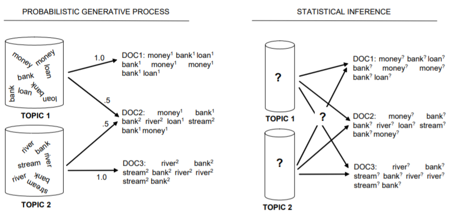
The Generation and Inference Process of a Topic Model

The generative process works by first selecting a topic according to some probability distribution, and then selecting a token from that topic according to another probability distribution. In contrast, the inference process starts with a set of documents and their tokens, but does not know which topic generated each token. What we need to infer is the probability distribution over topics for each document, as well as the probability distribution over words for each topic.

This inference cannot be made arbitrarily; it must be based on certain assumptions. Those assumptions are exactly the generative process of LDA (which is also why many introductions to LDA begin by describing its generative process).

Plate Representation of the LDA Generative Process

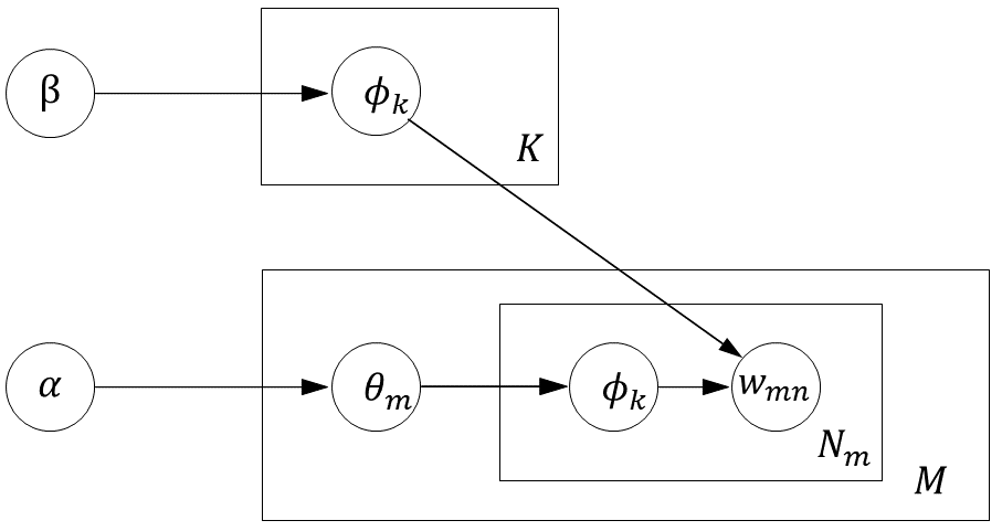
From the generative process above, we can see that the most important task is to estimate the parameters \(\Theta\) and \(\Phi\), namely \(\theta_{m}\) and \(\phi_{k}\). Both of these parameters can be estimated through sampling the topic assignment vector \(\textbf{z}\). In other words, if we can “reasonably” assign a topic to each word (that is, obtain several samples of \(\textbf{z}\)), then we can infer \(\theta\) and \(\phi\).

Thus, the problem becomes: given the observed data \(\textbf{w}\) and the prior hyperparameters \(\alpha\) and \(\beta\), how can we infer the distribution of \(\textbf{z}\) (and consequently sample from it)? That is, we want to compute:

\[p(\textbf{z}\vert\textbf{w},\alpha,\beta)\]

By Bayes’ rule, \(p(\textbf{z}\vert\textbf{w},\alpha,\beta)=\frac{p(\textbf{z},\textbf{w}\vert\alpha,\beta)}{p(\textbf{w}\vert\alpha,\beta)}\), the denominator is extremely difficult to estimate because of the high dimensionality and sparsity. Fortunately, when sampling \(\textbf{z}\), we only need the relative probabilities of \(\textbf{z}\) under different topic assignments. Therefore,

\[p(\textbf{z}\vert\textbf{w},\alpha,\beta)=\frac{p(\textbf{z},\textbf{w}\vert\alpha,\beta)}{p(\textbf{w}\vert\alpha,\beta)} \propto p(\textbf{z},\textbf{w}\vert\alpha,\beta)\]

So the key now is to compute \(p(\textbf{z},\textbf{w}\vert\alpha,\beta)\).

According to the generative process, given \(\alpha\) and \(\beta\), there are two latent variables, \(\theta\) and \(\phi\), between \(\textbf{z}\) and \(\textbf{w}\). Therefore, in order to obtain the above conditional probability, we need to integrate out these two latent variables (that is, compute the marginal probability):

\[p(\textbf{z},\textbf{w}\vert\alpha,\beta)=\int{\int{p(\textbf{z},\textbf{w},\theta,\phi\vert\alpha,\beta) \mathrm{d}\theta} \mathrm{d}\phi} = \int{\int{p(\phi\vert\beta)p(\theta\vert\alpha)p(\textbf{z}\vert\theta)p(\textbf{w}\vert\phi_{z})\mathrm{d}\theta}\mathrm{d}\phi} = \int{p(\textbf{z}\vert\theta)p(\theta\vert\alpha)\mathrm{d}\theta}\int{p(\textbf{w}\vert\phi_{z})p(\phi\vert\beta)\mathrm{d}\phi}\]

(that is, \(p(\textbf{z}\vert\alpha)p(\textbf{w}\vert\textbf{z},\beta)\))

We now derive these two terms separately.

2. Deriving the Two Terms

Let \(\theta_{mk}\) denote the probability that document \(m\) generates topic \(k\), and let \(n_{mk}\) denote the number of times topic \(k\) is assigned within document \(m\) in the corpus.

For the first term:

\[\begin{align*} p(\mathbf{z} \vert \alpha) &= \int p(\mathbf{z} \vert \theta) p(\theta \vert \alpha) \mathrm{d} \theta \\ &=\int \prod_{m=1}^{M} \frac{1}{\mathrm{~B}(\alpha)} \prod_{k=1}^{K} \theta_{m k}^{n_{m k}+\alpha_{k}-1} \mathrm{~d} \theta \\ &=\prod_{m=1}^{M} \frac{1}{\mathrm{~B}(\alpha)} \int \prod_{k=1}^{K} \theta_{m k}^{n_{m k}+\alpha_{k}-1} \mathrm{~d} \theta \\ &=\prod_{m=1}^{M} \frac{\mathrm{B}\left(n_{m}+\alpha\right)}{\mathrm{B}(\alpha)} \end{align*}\]

Here,

\[p(\mathbf{z} \vert \theta) = \prod_{m=1}^{M} \prod_{k=1}^{K} \theta_{m k}^{n_{m k}}\]

By assumption, \(\theta\) follows a Dirichlet distribution with parameter \(\alpha\). Therefore, the prior distribution of \(\theta\) is

\[p(\theta \vert \alpha)=\frac{\Gamma\left(\sum_{i=1}^{K} \alpha_{i}\right)}{\prod_{i=1}^{K} \Gamma\left(\alpha_{i}\right)} \prod_{i=1}^{K} \theta_{i}^{\alpha_{i}-1} =\frac{1}{\mathrm{~B}(\alpha)} \prod_{i=1}^{K} \theta_{i}^{\alpha_{i}-1} =\operatorname{Dir}(\theta \vert \alpha)\]

(see [1] for the derivation).

For the second term:

\[\begin{align*} p(\mathbf{w} \vert \mathbf{z}, \beta) &=\int p(\mathbf{w} \vert \mathbf{z}, \varphi) p(\varphi \vert \beta) \mathrm{d} \varphi \\ &=\int \prod_{k=1}^{K} \frac{1}{\mathrm{~B}(\beta)} \prod_{v=1}^{V} \varphi_{k v}^{n_{k v}+\beta_{v}-1} \mathrm{~d} \varphi \\ &=\prod_{k=1}^{K} \frac{1}{\mathrm{~B}(\beta)} \int \prod_{v=1}^{V} \varphi_{k v}^{n_{k v}+\beta_{v}-1} \mathrm{~d} \varphi \\ &=\prod_{k=1}^{K} \frac{\mathrm{B}\left(n_{k}+\beta\right)}{\mathrm{B}(\beta)} \end{align*}\]

where \(n_{k}=(n_{k1},n_{k2},\dots,n_{kV})\).

Here,

\[p(\mathbf{w} \vert \mathbf{z}, \phi) = \prod_{k=1}^{K} \prod_{v=1}^{V} \phi_{kv}^{n_{kv}}\]

Likewise, by assumption, \(\phi\) follows a Dirichlet distribution with parameter \(\beta\). Therefore, the prior distribution of \(\phi\) is

\[p(\phi_{k} \vert \beta)=\frac{\Gamma\left(\sum_{i=1}^{V} \beta_{i}\right)}{\prod_{i=1}^{V} \Gamma\left(\beta_{i}\right)} \prod_{v=1}^{V} \phi_{kv}^{\beta_{v}-1} =\frac{1}{\mathrm{~B}(\beta)} \prod_{v=1}^{V} \phi_{kv}^{\beta_{v}-1} =\operatorname{Dir}(\phi \vert \beta)\]

It follows that

\[p(\textbf{z},\textbf{w}\vert\alpha,\beta)=\prod_{d}\frac{B(n_{d,.}+\alpha)}{B(\alpha)} \prod_{k}\frac{B(n_{k,.}+\beta)}{B(\beta)}\]

that is,

\[p(\textbf{z} \vert\textbf{w},\alpha,\beta) \propto \prod_{d}\frac{B(n_{d,.}+\alpha)}{B(\alpha)} \prod_{k}\frac{B(n_{k,.}+\beta)}{B(\beta)}\]

3. Gibbs Sampling for LDA

So in principle, we can sample from \(p(\textbf{z}\vert\textbf{w},\alpha,\beta)\) according to the expression above. Direct sampling is possible, but it is highly inefficient in high-dimensional spaces. Therefore, we can instead use Gibbs sampling and sample one dimension at a time. To do that, we need to estimate \(p(z_{i}\vert\textbf{z}_{-i},\textbf{w},\alpha,\beta)\). It is easy to see that:

\[\begin{equation} p(z_{i}\vert\textbf{z}_{-i},\textbf{w},\alpha,\beta) =\frac{p(z_{i},\textbf{z}_{-i}\vert\textbf{w},\alpha,\beta)}{p(\textbf{z}_{-i}\vert\textbf{w},\alpha,\beta)} =\frac{p(\textbf{z}\vert\textbf{w},\alpha,\beta)}{p(\textbf{z}_{-i}\vert\textbf{w},\alpha,\beta)} \end{equation}\]

Let the denominator \(p(\textbf{z}_{-i},\textbf{w},\alpha,\beta)\) be denoted by \(Z_{i}\). \(Z_{i}\) is the marginal probability obtained after excluding the topic assignment at position \(i\). Note that \(Z_{i}\) is independent of the value of \(z_{i}\), because \(z_{i}\) has been excluded. That is,

\[Z_{z_i=t1}=Z_{z_i=t2},(t1 \neq t2)\]

Therefore,

\[p(z_{i}\vert\textbf{z}_{-i},\textbf{w},\alpha,\beta)=\frac{p(\textbf{z}\vert\textbf{w},\alpha,\beta)}{Z_{i}} \propto p(\textbf{z} \vert \textbf{w},\alpha,\beta) \propto \prod_{d}\frac{B(n_{d,.}+\alpha)}{B(\alpha)} \prod_{k}\frac{B(n_{k,.}+\beta)}{B(\beta)}\]

that is,

\[p(z_{i}\vert\textbf{z}_{-i},\textbf{w},\alpha,\beta) \propto \frac{n_{kv}+\beta_{v}}{\sum_{v=1}^{V}(n_{kv}+\beta_{v})} \frac{n_{mk}+\alpha_{k}}{\sum_{k=1}^{K}(n_{mk}+\alpha_{k})}\]

(for the derivation of this step, see ¹, p. 35).

At this point, the Gibbs sampling algorithm for LDA is almost immediate:

(The following is adapted from Li Hang’s Statistical Learning Methods ².)

Input: the word sequence of the corpus, \(\textbf{w}=\{\textbf{w}_{1},\textbf{w}_{2},\dots,\textbf{w}_{M}\}\)
Output: the topic sequence of the corpus, \(\textbf{z}=\{\textbf{z}_{1},\textbf{z}_{2},\dots,\textbf{z}_{M}\}\), and the estimated model parameters \(\theta\) and \(\phi\)
Hyperparameters: number of topics \(K\), and Dirichlet parameters \(\alpha\) and \(\beta\)

3.1 Initialization:

Let the “document-topic” count matrix be denoted by \(C_{MK}\), where \(C_{mk}\) represents the number of times topic \(k\) appears in document \(m\)
Let the “topic-word” count matrix be denoted by \(P_{KV}\), where \(P_{kv}\) represents the number of times word \(v\) appears under topic \(k\)
Let the “document-topic total” count vector be denoted by \((C_{1},C_{2},\dots,C_{M})\), where \(C_{m}\) represents the total number of topic assignments in document \(m\)
Let the “topic-word total” count vector be denoted by \((P_{1},P_{2},\dots,P_{K})\), where \(P_{k}\) represents the total number of words assigned to topic \(k\)

Initialize all the above variables to 0, and then perform the following steps:

For each document \(\textbf{w}_{m}\):

For each word \(w_{mn}\) in the document, where \(n=1,2,\dots,N_{m}\):

Sample a topic based on a multinomial distribution:

\(z_{mn}=z_{k}\sim Mult(\frac{1}{K})\)

\(C_{mk} += 1\), \(C_{m}+=1\), \(P_{kv}+=1\), \(P_{k}+=1\)

3.2 Training:

For each document \(\textbf{w}_{m}\):

For each word \(w_{mn}\) in the document:

Let the index of the current word in the vocabulary be \(v\), and let the topic index assigned to \(z_{mn}\) be \(k\)

\(C_{mk} -= 1\), \(C_{m}-=1\), \(P_{kv}-=1\), \(P_{k}-=1\)

Sample according to the conditional distribution:

\[p(z_{i}\vert\textbf{z}*{-i},\textbf{w},\alpha,\beta) \propto \frac{n*{kv}+\beta_{v}}{\sum_{v=1}^{V}(n_{kv}+\beta_{v})} \frac{n_{mk}+\alpha_{k}}{\sum_{k=1}^{K}(n_{mk}+\alpha_{k})}\]

Suppose the sampled topic is \(k^{\prime}\), and set \(z_{mn}=k^{\prime}\)

\(C_{mk^{\prime}} += 1\), \(C_{m}+=1\), \(P_{k^{\prime}v}+=1\), \(P_{k^{\prime}}+=1\)

Repeat the above steps until the burn-in period has passed. After convergence, obtain several samples of \(\textbf{z}\). These can then be used to estimate the parameters \(\theta\) and \(\phi\). Note that the estimation is based on the expectation of the distribution.

Finally, we obtain

\[\theta_{mk}=\frac{n_{mk}+\alpha_{k}}{\sum_{k=1}^{K}(n_{mk}+\alpha_{k})}\]

and

\[\phi_{kv}=\frac{n_{kv}+\beta_{v}}{\sum_{v=1}^{V}(n_{kv}+\beta_{v})}\]

That completes the algorithm.

When a new document arrives, we keep \(\phi\) fixed and update \(\theta\) in the same way as above, thereby obtaining the topic distribution of the document.

3.3 Estimating \(\theta\) and \(\phi\)

When estimating the parameter \(\theta\), according to the definition of LDA, we have

\[p\left(\theta_{m} \vert \mathbf{z}*{m}, \alpha\right)=\frac{1}{Z*{\theta_{m}}} \prod_{n=1}^{N_{m}} p\left(z_{m n} \vert \theta_{m}\right) p\left(\theta_{m} \vert \alpha\right)=\operatorname{Dir}\left(\theta_{m} \vert n_{m}+\alpha\right)\]

Then, by a property of the Dirichlet distribution (see [2]), we obtain

\[\theta_{mk}=\frac{n_{mk}+\alpha_{k}}{\sum_{k=1}^{K}(n_{mk}+\alpha_{k})}\]

When estimating the parameter \(\phi\), we have

\[p\left(\varphi_{k} \vert \mathbf{w}, \mathbf{z}, \beta\right)=\frac{1}{Z_{\varphi_{k}}} \prod_{i=1}^{I} p\left(w_{i} \vert \varphi_{k}\right) p\left(\varphi_{k} \vert \beta\right)=\operatorname{Dir}\left(\varphi_{k} \vert n_{k}+\beta\right)\]

Likewise, by the same property of the Dirichlet distribution, we obtain

\[\phi_{kv}=\frac{n_{kv}+\beta_{v}}{\sum_{v=1}^{V}(n_{kv}+\beta_{v})}\]

4. A Simple Python Implementation of LDA

Based on the algorithm above, it is fairly straightforward to write a program. It should be noted, however, that the implementation in this article is designed to be as easy to understand as possible, rather than heavily optimized. Here we use the TNEWS dataset as an example.

We first perform word segmentation, using HanLP as the tokenizer. We also remove special symbols and stop words, and use the hit_stopwords stop-word list.

Next, we implement the LDA model.

import re
import json
from pyhanlp import *

stopwords = set([line.strip('\n') for line in open('cn_stopwords.txt','r',encoding='utf-8').readlines()])

def tokenize(sent):
    pat = re.compile(r'[0-9!"#$$%&\'()*+,-./:;<=>?@—，。：★、￥…【】（）《》？“”‘’！\[\\\]^_`{|}~\u3000]+')
    return [t.word for t in HanLP.segment(sent) if pat.search(t.word)==None and t.word.strip()!='' and not (t.word in stopwords)]

def load_docs(filename,n_samples=-1):
    tokenized_docs = []
    with open(filename,'r',encoding='utf-8') as rfp:
        lines = [line.strip('\n') for line in rfp.readlines()]
        lines = lines if n_samples==-1 else lines[:n_samples]
        for i,line in enumerate(lines):
            sent = json.loads(line)['sentence']
            tokenized_docs.append(tokenize(sent))
            if i<100 and i%10==0:
                print(tokenize(sent))
    return tokenized_docs

trn_tokenized_docs = load_docs('tnews_public/train.json',n_samples=1000)
new_tokenized_docs = load_docs('tnews_public/dev.json',n_samples=1000)


'''
❯ python .\LDA.py
['上课时', '学生', '手机', '响', '个', '不停', '老师', '一怒之下', '把', '手机', '摔', '了', '家长', '拿', '发票', '让', '老师', '赔', '大家', '怎么', '
看待', '这种', '事']
['凌云', '研发', '的', '国产', '两', '轮', '电动车', '怎么样', '有', '什么', '惊喜']
['取名', '困难', '症', '患者', '皇马', '的', '贝尔', '第', '一个', '受害者', '就是', '他', '的', '儿子']
['葫芦', '都', '能', '做成', '什么', '乐器']
['中级会计', '考试', '每日', '一练']
['复仇者', '联盟', '中', '奇异', '博士', '为什么', '不', '用', '时间', '宝石', '跟', '灭', '霸', '谈判']
['拥抱', '编辑', '时代', '内容', '升级', '为', '产品', '海内外', '媒体', '如何', '规划', '下', '个', '十', '年']
['地球', '这', '是', '怎么', '了', '美国', '夏威夷', '群岛', '突发', '级', '地震', '游客', '紧急', '疏散']
['定安', '计划', '用', '三', '年', '时间', '修复', '全县', '处', '不', '可移动', '文物']
['军工', '已', '动真格', '中航', '科工', '占据', '着', '舞台', '正', '中央']

We would like it to provide the following interface:

lda_model = LDA(docs=tokenized_docs,K=20)

lda_model.train()

lda_model.add_docs(new_tokenized_docs)

tp_wd_dist = lda_model.topic_word_dist() 
# return [K,V] matrix

lda_model.show_topic_words()

doc_tp_dist = lda_model.get_corpus_dist()  
# return [M,K] matrix, where M = # of all the docs have feed in.

doc_tp_dist = lda_model.batch_inference(new_tokenized_docs) 
# return [M',K] matrix, where M' = # of new_tokenized_docs

tp_dist = lda_model.inference(new_tokenized_doc) 
# return [1,K] matrix

First comes the initialization part. This part is fairly straightforward to implement, and the functions of the key components are explained in the comments:

class LDA:
    def __init__(self,docs,K):
        # params: docs: tokenized sentence list, e.g. [['hello','world'],['nice','job'],...]
        # params: K: number of topics
        self.idx2token = []
        self.token2idx = {}
        self.M = len(docs) 
        self.K = K
        # Build vocabulary
        for doc in docs:
            for wd in doc:
                if not (wd in self.idx2token):
                    self.idx2token.append(wd)
        for idx,wd in enumerate(self.idx2token):
            self.token2idx[wd] = idx
        self.V = len(self.idx2token)
        print(f'Vocabulary length: {self.V}')

        # Initialize count matrix and vectors
        self.beta = np.ones(self.V) / self.V
        self.alpha = np.ones(self.K) / self.K
        self.matC = np.zeros((self.M,self.K))
        self.matP = np.zeros((self.K,self.V))
        self.vecC = np.zeros(self.M)
        self.vecP = np.zeros(self.K)
        self.zs = []
        self.k_ids = list(range(self.K)) # ids of topics
        self.v_docs = [] # mapping tokens in docs to their vocabulary index

        for m, doc in enumerate(docs):
            # sample topic ids for doc; 
            # np.random.choice is bootstrap sample method, which can generate array like [2,1,3,3]
            _zs = np.random.choice(self.k_ids,len(doc))
            self.zs.append(_zs)
            _idx = [self.token2idx[tk] for tk in doc]
            self.v_docs.append(_idx)
            for z,v in zip(_zs,_idx):
                self.matC[m,z] += 1
                self.matP[z,v] += 1
                self.vecP[z] += 1
            self.vecC[m] += len(doc)

Then comes the training part of LDA:

    def train(self,n_iter=100):
        for it in range(n_iter):
            print(f'Iteration {it} ...')
            for m,vdoc in enumerate(self.v_docs):
                for i,v in enumerate(vdoc):
                    z = self.zs[m][i]
                    self.matC[m][z] -= 1
                    self.vecC[m] -= 1
                    self.matP[z][v] -= 1
                    self.vecP[z] -= 1
                    fst_itm = lambda k: (self.matP[k][v]+self.beta[v])/(self.matP[k]+self.beta).sum()
                    scd_itm = lambda k: (self.matC[m][k]+self.alpha[k])/(self.matC[m]+self.alpha).sum()
                    _probs = np.array([fst_itm(k)*scd_itm(k) for k in self.k_ids])
                    probs = _probs / _probs.sum()
                    zp = np.random.choice(self.k_ids,p=probs)
                    self.zs[m][i] = zp
                    self.matC[m][zp] += 1
                    self.vecC[m] += 1
                    self.matP[zp][v] += 1
                    self.vecP[zp] += 1
        _theta = self.matC + self.alpha
        self.theta = _theta / _theta.sum(axis=1,keepdims=True)
        _phi = self.matP + self.beta
        self.phi = _phi / _phi.sum(axis=1,keepdims=True)

Suppose we have already trained the model and later obtain additional training data. We may then want to add an add_docs interface so that the model can continue training on top of the existing one. There are two possible implementation choices here. One is to keep the original vocabulary unchanged and update only the document set. This approach is simpler to implement and computationally more efficient. The other is to expand the vocabulary. This requires more computation, but it also reflects changes in the data more accurately.

    def add_docs(self,docs,n_iter=100):
        old_v = self.V
        # Update vocabulary
        for doc in docs:
            for tk in doc:
                if not (tk in self.idx2token):
                    self.idx2token.append(tk)
                    self.token2idx[tk] = len(self.idx2token)-1
        self.V = len(self.idx2token)
        self.beta = np.ones(self.V) / self.V # A convience way; other methods might be better?
        # Update idxes of docs: v_docs
        nv_docs = [[self.token2idx[tk] for tk in doc] for doc in docs]
        self.v_docs += nv_docs
        # Update shape of matC, matP, topic list: zs
        suf_matC = np.zeros((len(docs),self.K))
        suf_matP = np.zeros((self.K,self.V-old_v))
        self.matC = np.concatenate([self.matC,suf_matC],axis=0) # [M+M',K]
        self.matP = np.concatenate([self.matP,suf_matP],axis=1) # [K,V+V']
        vecC = []
        for m,doc in enumerate(nv_docs):
            _zs = np.random.choice(self.k_ids,len(doc))
            self.zs.append(_zs)
            for v,z in zip(doc,_zs):
                self.matC[m+self.M][z] += 1
                self.matP[z][v] += 1
                self.vecP[z] += 1
            vecC.append(len(doc))
        self.vecC = np.append(self.vecC,vecC)
        self.M = len(self.v_docs)

        # train for another more loops
        self.train(n_iter=n_iter)

When implementing the inference interface, since inference is essentially equivalent to adding new data and continuing the iterations until convergence, we can reuse the already implemented add_docs. The remaining interfaces are all auxiliary utilities and are relatively simple to implement, so I list them together here.

    def batch_inference(self,docs,n_iter=100):
        n_docs = len(docs)
        self.add_docs(docs,n_iter=n_iter)
        return self.get_corpus_dist()[-n_docs:]

    def inference(self,doc,n_iter=100):
        bth = [doc]
        dist = self.batch_inference(bth,n_iter=n_iter)
        return dist.squeeze()
        
    def get_corpus_dist(self):
        return self.theta

    def topic_word_dist(self):
        return self.phi

    def show_topic_words(self,n=20,show_weight=True):
        sorted_wghts = np.sort(-1 * self.phi,axis=1)[:,:n]*(-1) 
        top_idx = (-1 * self.phi).argsort(axis=1)[:,:n]
        suf = lambda wght: f'*{wght:.07f}' if show_weight else ''
        topic_words = [[f"{self.idx2token[idx]}{suf(wght)}" for idx,wght in zip(idxes,wghts)] for idxes,wghts in zip(top_idx,sorted_wghts)]
        for tp_wd in topic_words:
            print(tp_wd)
        return topic_words

Now let us apply the model to TNEWS. We set the number of iterations to 100, and inspect the model’s inferred document-topic distribution \(\theta\), as well as the top 20 topic words with the highest weights.

if __name__ == '__main__':
    N_Iter = 100
    print('Train on trn data ...')
    lda_model = LDA(docs=trn_tokenized_docs,K=20)
    lda_model.train(n_iter=N_Iter)
    tp_wd_dist = lda_model.topic_word_dist() # return [K,V] matrix
    print('tp_wd_dist:',tp_wd_dist)
    lda_model.show_topic_words(n=20)
    doc_tp_dist = lda_model.get_corpus_dist() # return [M,K] matrix, where M = # of all the docs have feed in.
    print('doc_tp_dist:',doc_tp_dist)

    print('='*40)
    print('Add Dev data')
    lda_model.add_docs(dev_tokenized_docs,n_iter=N_Iter)
    tp_wd_dist = lda_model.topic_word_dist() # return [K,V] matrix
    print('tp_wd_dist:',tp_wd_dist)
    lda_model.show_topic_words(n=20)
    doc_tp_dist = lda_model.get_corpus_dist() # return [M,K] matrix, where M = # of all the docs have feed in.
    print('doc_tp_dist:',doc_tp_dist)


    print('='*40)
    print('Inference on Test data')
    doc_tp_dist = lda_model.batch_inference(tst_tokenized_docs,n_iter=N_Iter) # return [M',K] matrix, where M' = # of new_tokenized_docs
    print('doc_tp_dist:',doc_tp_dist)
    new_tokenized_doc = tst_tokenized_docs[17]
    tp_dist = lda_model.inference(new_tokenized_doc,n_iter=N_Iter) # return [K] vector
    print('tp_dist:',tp_dist)
    
    
'''
>python LDA.py

Train on trn data ...
Vocabulary length: 4771

tp_wd_dist: [[6.29428422e-07 6.29428422e-07 6.29428422e-07 ... 6.29428422e-07
  6.29428422e-07 6.29428422e-07]
 [5.68020771e-07 5.68020771e-07 5.68020771e-07 ... 2.71059512e-03
  5.68020771e-07 5.68020771e-07]
 [5.64958665e-07 5.64958665e-07 4.58226674e-02 ... 5.64958665e-07
  5.64958665e-07 5.64958665e-07]
 ...
 [4.93175682e-07 4.93175682e-07 4.93175682e-07 ... 4.93175682e-07
  4.93175682e-07 4.93175682e-07]
 [5.22692431e-07 5.22692431e-07 5.22692431e-07 ... 5.22692431e-07
  5.22692431e-07 5.22692431e-07]
 [4.69954405e-07 4.69954405e-07 4.69954405e-07 ... 4.69954405e-07
  4.69954405e-07 4.69954405e-07]]
  
['年*0.0360367', '美国*0.0240247', '创新*0.0150156', '房产*0.0150156', '影响*0.0150156', '能力*0.0120126', '文化*0.0120126', '一个*0.0120126', '评价*0.0120126', '飞*0.0090096', '国*0.0090096', '娶*0.0090096', 'Q*0.0090096', '辆*0.0090096', '计划*0.0090096', '世界杯*0.0090096', '基地*0.0090096', '装备*0.0090096', '到来*0.0090096', '人性*0.0090096']
['四*0.0298109', '媒体*0.0162607', '建设*0.0162607', '楼市*0.0135507', '时间*0.0135507', '小镇*0.0135507', '西方*0.0108407', '成功*0.0108407', '时刻*0.0108407', '比特币*0.0108407', '爱*0.0108407', '首届*0.0108407', '赚钱*0.0108407', '农民*0.0108407', '没*0.0108407', '大战*0.0081306', '机遇*0.0081306', '沪
*0.0081306', '信*0.0081306', '专家*0.0081306']
['中*0.0512135', '手机*0.0458227', '太*0.0269547', '詹姆斯*0.0188685', '送*0.0161731', '科技*0.0134777', '里*0.0134777', '问题*0.0134777', '已经*0.0134777', '不能*0.0134777', '家长*0.0107822', '万*0.0107822', '万元*0.0107822', '路*0.0107822', '学会*0.0107822', '项*0.0107822', '农业*0.0080868', '制造*0.0080868', '幸福*0.0080868', '思考*0.0080868']
['一个*0.0488894', '中国*0.0444449', '三*0.0288894', '旅游*0.0266671', '新*0.0244449', '更*0.0200005', '没有*0.0200005', '即将*0.0177782', '经济*0.0133338', '重要*0.0111116', '产品*0.0111116', '喜欢*0.0111116', '老*0.0111116', '实力*0.0111116', '司机*0.0111116', '曝光*0.0111116', '请*0.0111116', '产业*0.0088894', '品牌*0.0088894', '难道*0.0088894']
['两*0.0474045', '做*0.0316032', '款*0.0248312', '王者*0.0203165', '俄*0.0180592', '开*0.0158018', '地球*0.0135445', '推荐*0.0135445', '孩子*0.0135445', 
'成*0.0112872', '投资*0.0112872', '值得*0.0112872', '要求*0.0112872', '谢娜*0.0090298', '区别*0.0090298', '首发*0.0090298', '重*0.0090298', '型*0.0090298', '见过*0.0090298', '先*0.0090298']
['现在*0.0473543', '历史*0.0222847', '房价*0.0167137', '儿子*0.0167137', '进*0.0167137', '举行*0.0167137', '元*0.0139282', '发*0.0111426', '梦*0.0111426', '航母*0.0111426', '联想*0.0083571', '逆袭*0.0083571', '周*0.0083571', '旗*0.0083571', '行情*0.0083571', '红毯*0.0083571', '再次*0.0083571', '收入*0.0083571', '现场*0.0083571', '风险*0.0083571']
['五*0.0294845', '到底*0.0196565', '网友*0.0171995', '核*0.0171995', '协议*0.0147425', '小米*0.0147425', '联*0.0147425', '地方*0.0147425', '微信*0.0122855', '亿*0.0122855', '伊*0.0122855', '｜*0.0122855', '融资*0.0122855', '出现*0.0098285', '爆*0.0098285', '好玩*0.0098285', '阿里巴巴*0.0098285', '改变*0.0098285', '教*0.0098285', '申请*0.0098285']
['」*0.0329119', '第一*0.0303803', '特朗普*0.0303803', '岁*0.0253170', '成功*0.0151904', '复*0.0151904', '上市*0.0126588', '油*0.0126588', '跑*0.0126588', '称*0.0126588', '印度*0.0101271', '智能*0.0101271', '电*0.0101271', '接*0.0101271', '参加*0.0101271', '进口*0.0101271', '电子*0.0101271', '上映*0.0075955', '获得*0.0075955', '号*0.0075955']
['会*0.0410262', '说*0.0333339', '使用*0.0179493', '位*0.0179493', '买房*0.0128211', '月*0.0128211', '终于*0.0128211', '便宜*0.0128211', '价格*0.0128211', '卡*0.0128211', '低*0.0102569', '酒*0.0102569', '主播*0.0102569', '苹果*0.0102569', '腿*0.0076928', '游*0.0076928', '高校*0.0076928', '竟然*0.0076928', '晋级*0.0076928', '分*0.0076928']
['亿*0.0453339', '美*0.0373339', '点*0.0320006', '没*0.0186672', '事件*0.0160006', '事*0.0160006', '版*0.0133339', '发明*0.0133339', '走*0.0133339', '猪*0.0133339', '恒大*0.0106672', '手游*0.0106672', '怒*0.0106672', '角色*0.0106672', '取消*0.0106672', '无数*0.0106672', '导弹*0.0106672', '响*0.0106672', '穿*0.0080006', '海南*0.0080006']
['中国*0.0316032', '看待*0.0316032', '俄罗斯*0.0293458', '学生*0.0225738', '发展*0.0203165', '级*0.0203165', '里*0.0203165', '老师*0.0180592', '知道*0.0158018', '普京*0.0158018', '种*0.0158018', '是否*0.0158018', '生活*0.0158018', '轮*0.0135445', '公司*0.0135445', '古代*0.0135445', '这种*0.0135445', '片*0.0112872', '最好*0.0112872', '故事*0.0112872']
['荣耀*0.0243249', '比较*0.0243249', '教育*0.0216222', '首*0.0189195', '应该*0.0162168', '全球*0.0162168', '国产*0.0162168', 'G*0.0135141', '数据*0.0135141', '行业*0.0135141', '半*0.0108114', '一战*0.0108114', '反*0.0108114', '南昌*0.0108114', '偶遇*0.0081087', '公布*0.0081087', '大爷*0.0081087', '听说*0.0081087', '发声*0.0081087', '创*0.0081087']
['年*0.0725005', '十*0.0475005', '日本*0.0400005', '汽车*0.0150005', '项目*0.0150005', '银行*0.0125005', '选择*0.0125005', '实现*0.0125005', '晒*0.0125005', '地震*0.0125005', '女友*0.0100005', '国内*0.0100005', '山*0.0100005', '德国*0.0100005', '结婚*0.0100005', '微博*0.0100005', '张*0.0100005', '富士康*0.0075005', '史上*0.0075005', '互联网*0.0075005']
['会*0.0232564', 'A*0.0206724', '比赛*0.0155044', '原来*0.0129204', '腾讯*0.0129204', '发生*0.0129204', '济南*0.0129204', 'NBA*0.0129204', '活动*0.0129204', '方面*0.0103365', '直接*0.0103365', '水平*0.0103365', '没有*0.0103365', '·*0.0103365', '仅*0.0103365', '功能*0.0103365', '尴尬*0.0077525', '陕西*0.0077525', '令狐冲*0.0077525', '棋牌*0.0077525']
['上联*0.0362817', '下联*0.0362817', '城市*0.0294789', '三*0.0181411', '游客*0.0158735', '公里*0.0158735', '深圳*0.0158735', '勇士*0.0136059', '千*0.0136059', '火箭*0.0136059', '座*0.0136059', '上海*0.0113383', '泰山*0.0113383', '黄山*0.0113383', '造*0.0113383', '赵本山*0.0113383', '分钟*0.0113383', '正确
*0.0090708', '内容*0.0090708', '有人*0.0090708']
['美国*0.0388606', '伊朗*0.0310886', '车*0.0284980', '真的*0.0207259', '超*0.0155446', '名*0.0129539', '叙利亚*0.0129539', '小时*0.0129539', '最多*0.0129539', '空袭*0.0129539', '面临*0.0129539', '适合*0.0129539', '外*0.0103632', '升级*0.0103632', '进入*0.0103632', '鸡*0.0077726', '退出*0.0077726', '季*0.0077726', '大型*0.0077726', '计算机*0.0077726']
['买*0.0467039', '万*0.0439566', '国家*0.0247259', '中*0.0219786', '米*0.0192313', '吃*0.0164841', '出*0.0164841', '行*0.0137368', '知道*0.0137368', '最 
后*0.0137368', '启动*0.0137368', '现身*0.0109896', '河南*0.0109896', '战争*0.0109896', '作品*0.0109896', '时*0.0109896', '抵达*0.0109896', '文明*0.0109896', '工作*0.0082423', '每月*0.0082423']
['中国*0.0635299', '世界*0.0447064', '高*0.0211770', '链*0.0188240', '成为*0.0188240', '原因*0.0188240', '前*0.0164711', '区块*0.0164711', '美元*0.0164711', '技术*0.0141181', '曾经*0.0141181', '今年*0.0117652', '平台*0.0117652', '认为*0.0094123', '太空*0.0094123', '唯一*0.0094123', '无法*0.0094123', '北京
*0.0094123', '解说*0.0094123', '排名*0.0094123']
['日*0.0374070', '游戏*0.0374070', '「*0.0349132', '钱*0.0224444', '以色列*0.0174569', '农村*0.0174569', '省*0.0149631', '建*0.0124694', '天*0.0124694', 
'东西*0.0124694', '市场*0.0124694', '考*0.0099756', '泰国*0.0099756', '创业*0.0099756', '快*0.0099756', '车*0.0099756', '处理*0.0074818', '机器人*0.0074818', '届*0.0074818', '灯*0.0074818']
['次*0.0336328', '会*0.0291485', '联盟*0.0246641', '英雄*0.0246641', '玩*0.0201798', '需要*0.0201798', '股*0.0134534', '复仇者*0.0134534', '冠军*0.0134534', '战场*0.0112112', '回应*0.0112112', '很多*0.0089691', '获*0.0089691', '赛*0.0089691', '带*0.0089691', '看到*0.0089691', '贷款*0.0089691', '虎牙*0.0089691', '怕*0.0089691', '央视*0.0089691']

doc_tp_dist: [[0.00294118 0.00294118 0.47352941 ... 0.00294118 0.00294118 0.00294118]
 [0.065625   0.003125   0.003125   ... 0.065625   0.003125   0.003125  ]
 [0.00454545 0.00454545 0.00454545 ... 0.00454545 0.36818182 0.00454545]
 ...
 [0.00714286 0.72142857 0.00714286 ... 0.00714286 0.00714286 0.00714286]
 [0.00833333 0.00833333 0.00833333 ... 0.00833333 0.00833333 0.00833333]
 [0.00625    0.00625    0.00625    ... 0.13125    0.00625    0.00625   ]]
'''

Intuitively, from the results we can see that the topic words of some topics do exhibit a certain degree of semantic coherence, while others are more obscure. As for quantitatively evaluating the quality of topic modeling results, that is a much broader topic and will not be discussed in this article. If we switch to a different stop-word list—for example, replacing the stop words with baidu_stopwords—the results also change significantly. This suggests that the performance of topic models is highly sensitive to the choice of stop-word list, so the domain of the data should be carefully considered when selecting stop words.

References

马晨. 《LDA漫游指南》. https://www.epubit.com/bookDetails?id=N23066 ↩
李航. 《统计学习方法》. https://book.douban.com/subject/33437381/ ↩