From Gaussian Priors to Invertible Networks: Understanding NICE and Flow Models
Background
This post is an introduction to and implementation of the paper NICE: Non-linear Independent Components Estimation. It is also one of the foundational papers behind Glow, and in many ways can be regarded as the cornerstone on which Glow was built.
Difficult Distributions
As is well known, the mainstream generative models today include VAEs and GANs. But in fact, besides these two, there is another major family: flow-based models. The word flow can be translated literally, though we will introduce its meaning more carefully later.
Historically, flow models are just as old as VAEs and GANs, yet they have remained relatively obscure. In my view, one reason is that flow lacks an intuitive narrative like GAN’s “counterfeiter vs. detective.” Flow models are more mathematical in nature, and early results were not especially impressive despite their heavy computational cost, so they were less appealing at first glance. Today, however, OpenAI’s remarkably strong flow-based Glow model will likely attract much more attention to this line of research.
At its core, a generative model aims to fit the observed data using a probability model we can explicitly specify. In other words, we need to write down a parameterized distribution \(q_{\boldsymbol{\theta}}(\boldsymbol{x}).\) However, a neural network is a universal function approximator, not a universal distribution approximator. In principle, it can approximate arbitrary functions, but it cannot directly represent an arbitrary probability distribution, because a valid distribution must satisfy non-negativity and normalization. As a result, the distributions we can write down directly are usually either discrete distributions or continuous Gaussian distributions.
Strictly speaking, images should be viewed as discrete distributions, since they consist of a finite number of pixels and each pixel takes values from a finite discrete set. This line of thinking leads to models such as PixelRNN, which we may call autoregressive flows. Their major drawback is that they cannot be parallelized, making them computationally very expensive. For this reason, we would often prefer to model images using continuous distributions. And of course, images are just one example—many real-world datasets are continuous, so studying continuous distributions is important in its own right.
Different Ways Around the Problem
This brings us to the main difficulty: for continuous variables, the most convenient distribution we can write down is often just a Gaussian. In many cases, for tractability, we further assume that the components are independent, which leaves us with only a tiny corner of the space of all continuous distributions. Clearly, that is far from sufficient.
To overcome this, we can construct richer distributions through integration: \(q(\boldsymbol{x})=\int q(\boldsymbol{z})q_{\boldsymbol{\theta}}(\boldsymbol{x}|\boldsymbol{z}) , d\boldsymbol{z}\tag{1}\)
Here, \(q(\boldsymbol{z})\) is usually chosen as a standard Gaussian, while \(q_{\boldsymbol{\theta}}(\boldsymbol{x}|\boldsymbol{z})\) can be any conditional Gaussian distribution or a Dirac delta distribution. This integral form can represent very complicated distributions. In theory, it is expressive enough to approximate arbitrary distributions.
Now that we have a flexible family of distributions, we need to learn the parameters \(\theta\). The standard approach is maximum likelihood. If the true data distribution is denoted by \(\tilde{p}(\boldsymbol{x}),\) then we want to maximize \(\mathbb{E}_{\boldsymbol{x}\sim \tilde{p}(\boldsymbol{x})} \big[\log q(\boldsymbol{x})\big].\tag{2}\)
The problem is that \(q_{\boldsymbol{\theta}}(\boldsymbol{x})\) is defined through an integral, and whether this integral can be computed tractably is another matter entirely.
At this point, researchers took very different routes. VAE and GAN each avoid this difficulty in their own way. A VAE does not optimize the objective in (2) directly; instead, it optimizes a lower bound, which makes it fundamentally approximate and can limit generation quality. GANs, on the other hand, bypass the likelihood computation through adversarial training. This preserves the sharpness of the model and is one reason GANs can generate such impressive samples. That said, GANs are not perfect either, so it remains meaningful to explore alternative solutions.
Facing the Probability Integral Head-On
Flow models choose the hard road: compute the integral directly.
More specifically, a flow model chooses \(q(\boldsymbol{x}|\boldsymbol{z})\) to be a Dirac delta distribution \(\delta(\boldsymbol{x}-\boldsymbol{g}(\boldsymbol{z})),\) with the additional requirement that \(\boldsymbol{g}\) be invertible, i.e. \(\boldsymbol{x}=\boldsymbol{g}(\boldsymbol{z}) \Leftrightarrow \boldsymbol{z} = \boldsymbol{f}(\boldsymbol{x}).\tag{3}\)
For invertibility to hold in the mathematical sense, \(\boldsymbol{x}\) and \(\boldsymbol{z}\) must have the same dimensionality. Assuming the forms of \(\boldsymbol{f}\) and \(\boldsymbol{g}\) are known, computing \(q(\boldsymbol{x})\) from (1) amounts to applying the change of variables \(\boldsymbol{z}=\boldsymbol{f}(\boldsymbol{x}).\) That is, we start from the standard Gaussian \(q(\boldsymbol{z}) = \frac{1}{(2\pi)^{D/2}}\exp\left(-\frac{1}{2} \Vert \boldsymbol{z}\Vert^2\right),\tag{4}\) where \(D\) is the dimensionality of \(\boldsymbol{z}\), and then transform variables using \(\boldsymbol{z}=\boldsymbol{f}(\boldsymbol{x}).\)
Importantly, a change of variables for probability densities is not obtained by simply replacing \(\boldsymbol{z}\) with \(\boldsymbol{f}(\boldsymbol{x})\). One must also multiply by the absolute value of the Jacobian determinant: \(q(\boldsymbol{x}) = \frac{1}{(2\pi)^{D/2}}\exp\left(-\frac{1}{2}\big\Vert \boldsymbol{f}(\boldsymbol{x})\big\Vert^2\right)\left|\det\left[\frac{\partial \boldsymbol{f}}{\partial \boldsymbol{x}}\right]\right|.\tag{5}\)
So, for \(\boldsymbol{f}\) we need two things:
- It must be invertible, and its inverse must be easy to compute (since its inverse \(\boldsymbol{g}\) is precisely the generative model we want);
- Its Jacobian determinant must be easy to compute.
Then \(\log q(\boldsymbol{x}) = -\frac{D}{2}\log (2\pi) -\frac{1}{2}\big\Vert \boldsymbol{f}(\boldsymbol{x})\big\Vert^2 + \log \left|\det\left[\frac{\partial \boldsymbol{f}}{\partial \boldsymbol{x}}\right]\right|,\tag{6}\) and this objective is tractable.
Moreover, because \(\boldsymbol{f}\) is easy to invert, once training is complete we can sample a random \(\boldsymbol{z}\) and generate a sample through \(\boldsymbol{f}^{-1}(\boldsymbol{z})=\boldsymbol{g}(\boldsymbol{z}),\) which gives us a generative model.
Flow
We have now outlined both the key idea and the main challenge behind flow models. Next, let us look at how flow models address this challenge in detail. Since this post focuses on the first paper, NICE: Non-linear Independent Components Estimation, we will refer to the model here specifically as NICE.
Coupling Layers by Partition
In practice, computing determinants is usually harder than inverting functions, so it makes sense to start from requirement 2 above. Anyone familiar with linear algebra knows that triangular matrices are especially convenient: the determinant of a triangular matrix is simply the product of its diagonal entries. Therefore, we should try to design \(\boldsymbol{f}\) so that its Jacobian is triangular.
NICE uses a very elegant construction. It splits the \(D\)-dimensional input \(\boldsymbol{x}\) into two parts, \(\boldsymbol{x}_1\) and \(\boldsymbol{x}_2\), and defines the transformation \(\begin{aligned} &\boldsymbol{h}_1 = \boldsymbol{x}_1\\ &\boldsymbol{h}_2 = \boldsymbol{x}_2 + \boldsymbol{m}(\boldsymbol{x}_{1}) \end{aligned}\tag{7}\)
Here \(\boldsymbol{x}_1\) and \(\boldsymbol{x}_2\) are a partition of \(\boldsymbol{x}\), and \(\boldsymbol{m}\) is an arbitrary function of \(\boldsymbol{x}_1\). In other words, we split \(\boldsymbol{x}\) into two parts, transform it according to the formula above, and obtain a new variable \(\boldsymbol{h}\). This is called an additive coupling layer.
Without loss of generality, we can permute the coordinates of \(\boldsymbol{x}\) so that \(\boldsymbol{x}_1 = \boldsymbol{x}_{1:d}\) contains the first \(d\) components, and \(\boldsymbol{x}_2 = \boldsymbol{x}_{d+1:D}\) contains components \(d+1,\ldots,D\).
It is easy to see that the Jacobian matrix \(\left[\frac{\partial \boldsymbol{h}}{\partial \boldsymbol{x}}\right]\) is triangular, with all diagonal entries equal to 1. In block form,
\[\left[\frac{\partial \boldsymbol{h}}{\partial \boldsymbol{x}}\right]= \begin{pmatrix} \mathbb{I}_{1:d} & \mathbb{O} \\ \left[\frac{\partial \boldsymbol{m}}{\partial \boldsymbol{x}_{1}}\right] & \mathbb{I}_{d+1:D} \end{pmatrix}.\tag{8}\]Therefore, the Jacobian determinant is 1, and its log-determinant is 0. This completely eliminates the determinant-computation problem.
At the same time, the transformation in (7) is invertible, with inverse
\[\begin{aligned} &\boldsymbol{x}_1 = \boldsymbol{h}_1\\ &\boldsymbol{x}_2 = \boldsymbol{h}_2 - \boldsymbol{m}(\boldsymbol{h}_{1}) \end{aligned}\tag{9}\]A Flow of Small Steps
The transformation above is quite remarkable: it is invertible, and the inverse is just as simple, with essentially no extra computational cost. Still, we should notice that in (7), the first part is left unchanged, so a single transformation cannot be highly nonlinear. To obtain a sufficiently expressive model, we need to compose many such simple transformations:
\[\boldsymbol{x} = \boldsymbol{h}^{(0)} \leftrightarrow \boldsymbol{h}^{(1)} \leftrightarrow \boldsymbol{h}^{(2)} \leftrightarrow \dots \leftrightarrow \boldsymbol{h}^{(n-1)} \leftrightarrow \boldsymbol{h}^{(n)} = \boldsymbol{z}.\tag{10}\]Each step is an additive coupling layer. This sequence of transformations resembles water flowing in a stream: small changes accumulate into a powerful overall transformation. That is why the whole procedure is called a flow.
By the chain rule,
\[\left[\frac{\partial \boldsymbol{z}}{\partial \boldsymbol{x}}\right] = \left[\frac{\partial \boldsymbol{h}^{(n)}}{\partial \boldsymbol{h}^{(n-1)}}\right] \left[\frac{\partial \boldsymbol{h}^{(n-1)}}{\partial \boldsymbol{h}^{(n-2)}}\right] \dots \left[\frac{\partial \boldsymbol{h}^{(1)}}{\partial \boldsymbol{h}^{(0)}}\right].\tag{11}\]Since the determinant of a product equals the product of determinants, and every layer is an additive coupling layer with determinant 1, we obtain
\[\det \left[\frac{\partial \boldsymbol{z}}{\partial \boldsymbol{x}}\right] = \det\left[\frac{\partial \boldsymbol{h}^{(n)}}{\partial \boldsymbol{h}^{(n-1)}}\right] \det\left[\frac{\partial \boldsymbol{h}^{(n-1)}}{\partial \boldsymbol{h}^{(n-2)}}\right] \dots \det\left[\frac{\partial \boldsymbol{h}^{(1)}}{\partial \boldsymbol{h}^{(0)}}\right] =1.\](With permutations introduced later, the determinant can become \(-1\), but its absolute value remains 1.) So the determinant remains trivial to handle.
Progress Through Alternation
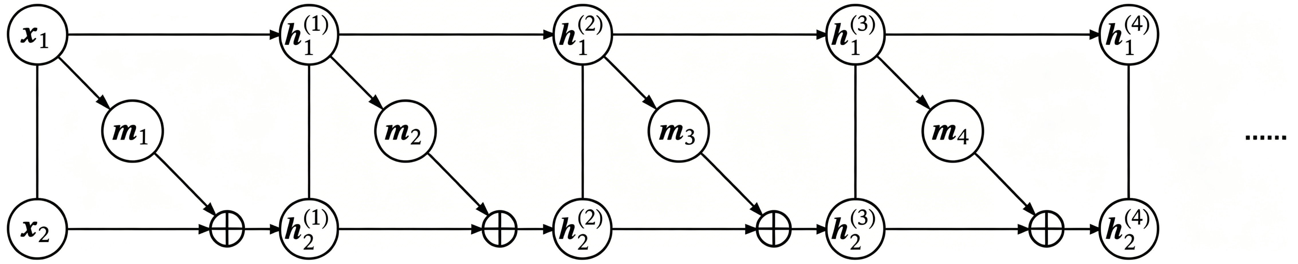
One subtle but important point: if the coupling order never changes, i.e.
\[\begin{array}{ll} \begin{aligned} &\boldsymbol{h}^{(1)}_{1} = \boldsymbol{x}_{1}\\ &\boldsymbol{h}^{(1)}_{2} = \boldsymbol{x}_{2} + \boldsymbol{m}_1(\boldsymbol{x}_{1}) \end{aligned} & \begin{aligned} &\boldsymbol{h}^{(2)}_{1} = \boldsymbol{h}^{(1)}_{1}\\ &\boldsymbol{h}^{(2)}_{2} = \boldsymbol{h}^{(1)}_{2} + \boldsymbol{m}_2\big(\boldsymbol{h}^{(1)}_{1}\big) \end{aligned} \\[0.75em] \begin{aligned} &\boldsymbol{h}^{(3)}_{1} = \boldsymbol{h}^{(2)}_{1}\\ &\boldsymbol{h}^{(3)}_{2} = \boldsymbol{h}^{(2)}_{2} + \boldsymbol{m}_3\big(\boldsymbol{h}^{(2)}_{1}\big) \end{aligned} & \begin{aligned} &\boldsymbol{h}^{(4)}_{1} = \boldsymbol{h}^{(3)}_{1}\\ &\boldsymbol{h}^{(4)}_{2} = \boldsymbol{h}^{(3)}_{2} + \boldsymbol{m}_4\big(\boldsymbol{h}^{(3)}_{1}\big) \end{aligned} \\ & \qquad \cdots \end{array}\tag{12}\]then in the end we still have \(\boldsymbol{z}_1 = \boldsymbol{x}_1\). The first part remains trivial, as shown below.
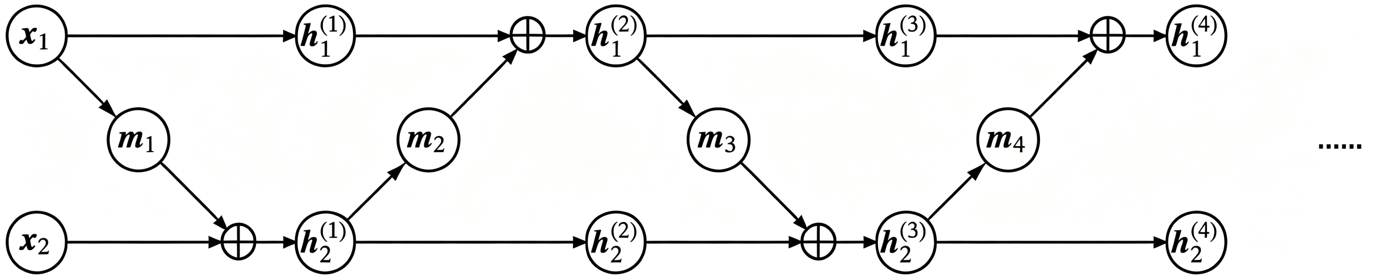
To obtain a nontrivial transformation, we can permute or reverse the input dimensions before each additive coupling layer, or simply swap the two partitions so that information can mix thoroughly. For example,
\[\begin{array}{ll} \begin{aligned} &\boldsymbol{h}^{(1)}_{1} = \boldsymbol{x}_{1}\\ &\boldsymbol{h}^{(1)}_{2} = \boldsymbol{x}_{2} + \boldsymbol{m}_1(\boldsymbol{x}_{1}) \end{aligned} & \begin{aligned} &\boldsymbol{h}^{(2)}_{1} = \boldsymbol{h}^{(1)}_{1} + \boldsymbol{m}_2\big(\boldsymbol{h}^{(1)}_{2}\big)\\ &\boldsymbol{h}^{(2)}_{2} = \boldsymbol{h}^{(1)}_{2} \end{aligned} \\[0.75em] \begin{aligned} &\boldsymbol{h}^{(3)}_{1} = \boldsymbol{h}^{(2)}_{1}\\ &\boldsymbol{h}^{(3)}_{2} = \boldsymbol{h}^{(2)}_{2} + \boldsymbol{m}_3\big(\boldsymbol{h}^{(2)}_{1}\big) \end{aligned} & \begin{aligned} &\boldsymbol{h}^{(4)}_{1} = \boldsymbol{h}^{(3)}_{1} + \boldsymbol{m}_4\big(\boldsymbol{h}^{(3)}_{2}\big)\\ &\boldsymbol{h}^{(4)}_{2} = \boldsymbol{h}^{(3)}_{2} \end{aligned} \\ & \qquad \cdots \end{array}\tag{13}\]as illustrated below.
Scaling Layer
Earlier we pointed out that flow models are based on invertible transformations, so once training is complete, we obtain both a generative model and an encoder. But precisely because the transformation is invertible, the latent variable \(\boldsymbol{z}\) has the same dimensionality as the input \(\boldsymbol{x}\).
Now, when we specify \(\boldsymbol{z}\) to follow a Gaussian distribution, it occupies the entire \(D\)-dimensional space, where \(D\) is the size of \(\boldsymbol{x}\). But although \(\boldsymbol{x}\) has \(D\) coordinates, it may not actually fill the whole \(D\)-dimensional space. For example, an MNIST image has 784 pixels, but some pixels are always zero in both the training and test sets, which suggests the true intrinsic dimensionality is much lower than 784.
In other words, flow models based on invertible transformations naturally suffer from a severe dimension waste problem: the input data may not lie on a full \(D\)-dimensional manifold, yet we still force it to be encoded into one. Is that really reasonable?
To address this, NICE introduces a scaling layer, which rescales each feature in the final encoding: \(\boldsymbol{z} = \boldsymbol{s}\otimes \boldsymbol{h}^{(n)},\) where \(\boldsymbol{s} = (\boldsymbol{s}_1,\boldsymbol{s}_2,\dots,\boldsymbol{s}_D)\) is also a learnable parameter vector, with nonnegative entries. This vector can indicate the importance of each dimension: smaller values correspond to more important dimensions, while larger values suggest less important ones, potentially close to ignorable. In effect, this layer compresses the manifold.
The Jacobian determinant of this scaling layer is no longer 1. Its Jacobian matrix is diagonal: \(\left[\frac{\partial \boldsymbol{z}}{\partial \boldsymbol{h}^{(n)}}\right] = \text{diag}, (\boldsymbol{s}).\tag{14}\) Hence its determinant is \(\prod_i \boldsymbol{s}_i\). According to (6), the log-likelihood becomes
\[\log q(\boldsymbol{x}) \sim -\frac{1}{2}\big\Vert \boldsymbol{s}\otimes \boldsymbol{f} (\boldsymbol{x})\big\Vert^2 + \sum_i \log \boldsymbol{s}_i.\tag{15}\]Why does this scaling layer reflect feature importance? It helps to reinterpret it from another perspective.
Initially, we assume that \(\boldsymbol{z}\) follows a standard normal prior, so each dimension has variance 1. But in fact, we can also make the variances of the prior trainable. After training, some variances may become small while others remain large. A small variance means that the feature has little spread; if the variance becomes 0, that feature collapses to the constant mean 0, so the distribution along that dimension reduces to a single point. This effectively reduces the dimensionality of the manifold by one.
Instead of (4), let us write a Gaussian with per-dimension variances:
\[q(\boldsymbol{z}) = \frac{1}{(2\pi)^{D/2}\prod\limits_{i=1}^D \boldsymbol{\sigma}_i}\exp\left(-\frac{1}{2}\sum_{i=1}^D \frac{\boldsymbol{z}_i^2}{\boldsymbol{\sigma}_i^2}\right).\tag{16}\]Substituting the flow model \(\boldsymbol{z}=\boldsymbol{f}(\boldsymbol{x})\) into the above, and taking logs as in (6), we obtain
\[\log q(\boldsymbol{x}) \sim -\frac{1}{2}\sum_{i=1}^D \frac{\boldsymbol{f}_i^2(\boldsymbol{x})}{\boldsymbol{\sigma}_i^2} - \sum_{i=1}^D \log \boldsymbol{\sigma}_i.\tag{17}\]Comparing (15) and (17), we see that \(\boldsymbol{s}_i=1/\boldsymbol{\sigma}_i.\) So the scaling layer is equivalent to making the variances (or standard deviations) of the prior trainable. If a variance becomes sufficiently small, we may regard the corresponding manifold dimension as having collapsed to a point, which implicitly introduces the possibility of dimensionality reduction.
Disentangling Features
If we choose the prior to be a Gaussian with independent components, does that offer any benefit beyond convenient sampling?
In a flow model, \(\boldsymbol{f}^{-1}\) is the generative model used to produce random samples, and \(\boldsymbol{f}\) acts as an encoder. But unlike an ordinary autoencoder, which compresses high-dimensional data into a lower-dimensional latent representation to force the network to extract useful information, a flow model is fully invertible. There is no information loss. So what is the value of such an encoder?
This brings us to a deeper question: what makes a good representation?
In everyday life, we often describe things along abstract dimensions such as “height,” “weight,” “beauty,” or “wealth.” The point is that when we say someone is tall, that does not necessarily imply they are overweight or underweight, nor does it imply they are rich or poor. Ideally, these dimensions should not strongly determine one another; otherwise they would be redundant. So, a good representation should ideally consist of features that are independent, or at least as disentangled as possible, so that each dimension carries its own meaning.
This is exactly the advantage of choosing a prior with independent Gaussian components. Because the components are independent, when we encode the original input through \(\boldsymbol{f}\) and obtain \(\boldsymbol{z}=\boldsymbol{f}(\boldsymbol{x}),\) we have reason to interpret the different dimensions of \(\boldsymbol{z}\) as disentangled latent factors.
This is also what the name NICE—Non-linear Independent Components Estimation—refers to.
Conversely, because the dimensions of \(\boldsymbol{z}\) are independent, in principle we can vary a single latent dimension while keeping the others fixed and observe how the generated image changes, thereby uncovering the semantic meaning of that dimension.
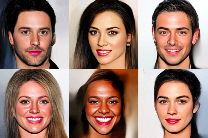
Similarly, we can interpolate between the encodings of two images—for example, by taking weighted averages—and obtain smoothly varying generated samples. This idea is explored much more fully in later models such as Glow. Since this post only reports MNIST experiments, however, we will not emphasize this aspect here.
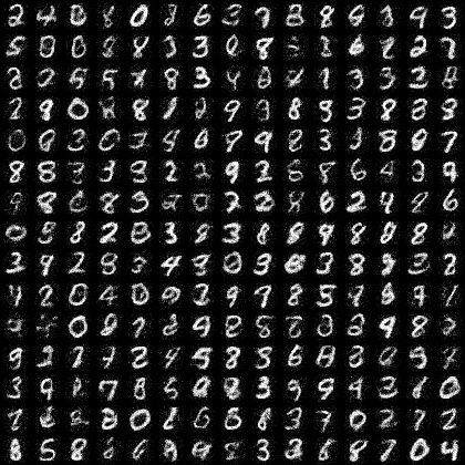
Experiments
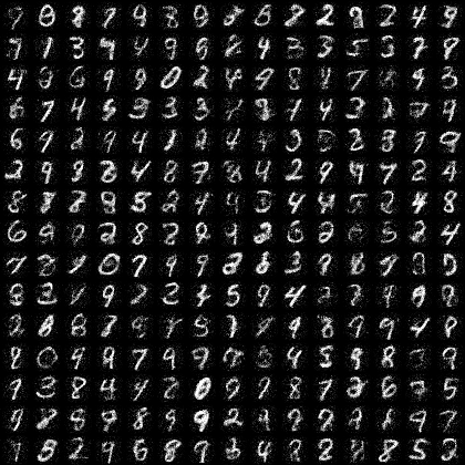
Here we reproduce the MNIST experiment from the NICE paper using Keras.
Model Details
Let us first summarize the components of the NICE model.
NICE is a type of flow model built from multiple additive coupling layers. Each additive coupling layer is defined as in (7), and its inverse is given by (9). Before each coupling, the input dimensions are reversed or permuted so that information mixes sufficiently. Finally, a scaling layer is added at the end. The final loss is the negative of (15).
Each additive coupling layer splits the input into two parts. NICE uses an alternating partition: the even-indexed coordinates form one part, and the odd-indexed coordinates form the other. Each function \(\boldsymbol{m}(\boldsymbol{x})\) is implemented as a multilayer fully connected network with 5 hidden layers, each containing 1000 units and using ReLU activations. NICE stacks a total of 4 additive coupling layers.
As for the input, the original pixel values in the range 0–255 are first rescaled to 0–1 by dividing by 255. Then uniform noise from the interval \([-0.01, 0]\) is added. Adding noise can effectively reduce overfitting and improve sample quality. It can also be seen as a way to alleviate the dimension-waste problem, because MNIST images by themselves do not really occupy the full 784-dimensional space, while the injected noise increases the effective dimensionality.
Readers may wonder why the noise interval is \([-0.01,0]\) rather than \([0,0.01]\) or \([-0.005,0.005]\). In fact, from the perspective of the loss, these choices behave similarly, and replacing uniform noise with Gaussian noise also makes little difference. However, once noise is added during training, generated images will theoretically contain noise as well, which is not desirable. Using negative noise nudges the generated pixel values slightly toward the negative range, so we can remove part of the noise afterward simply by applying a clip operation. This is just a small trick for MNIST and not a particularly important one.
Reference Code
Here is my Keras reference implementation:
In my experiments, the model reaches its best performance within 20 epochs. Each epoch takes about 11 seconds on a GTX 1070, and the final loss is around -2200.
Compared with the original paper, I made several modifications. For the additive coupling layer, I use (9) as the forward transformation and (7) as its inverse. Since \(m(x)\) uses ReLU activations, and ReLU outputs are nonnegative, these two choices are not exactly equivalent. Because the forward direction is the encoder and the inverse direction is the generator, using (7) as the inverse makes the generative model more inclined to produce positive values, which matches our target image domain well, since the desired pixel range is 0–1.
Annealing Parameter
Although at test time we ultimately want to sample from a standard normal distribution, for a trained model the ideal sampling variance is not necessarily exactly 1. In practice, it often fluctuates around 1 and is typically slightly smaller. The standard deviation used for final sampling is what we call the annealing parameter.
For example, in the reference implementation above, the annealing parameter is set to 0.75, which visually seems to give the best sample quality.
Conclusion
NICE is actually a fairly large model. Under the configuration described above, the number of parameters is approximately \(4 \times 5 \times 1000^2 = 2\times 10^7,\) that is, around 20 million parameters just to train a generative model on MNIST—which is rather extravagant.
Overall, NICE is conceptually simple and direct. The additive coupling itself is straightforward, and the transformation network \(\boldsymbol{m}\) is implemented using only large fully connected layers, without incorporating convolutions or other more sophisticated architectural ideas. So there is still plenty of room for exploration. Real NVP and Glow are two important successors that improve upon NICE, and their stories are best left for another time.
Enjoy Reading This Article?
Here are some more articles you might like to read next: